# Seeing Sound: Generative Techno and DSP in Pure NumPy
URL: https://www.msuiche.com/posts/seeing-sound-generative-techno-and-dsp-in-pure-numpy/
Date: 2026-04-13
Author: Matt Suiche
Tags: Techno, Acid, DSP, Generative, NumPy, Synthesis, Sound Design
> Building a complete generative techno engine and a reference-track analyzer in pure NumPy — from raw oscillators to 8 arranged-track genre presets. Covers DSP fundamentals, envelopes, LFOs, filters, sidechain, generative patterns, arrangement, reverse-engineering real tracks, and seeing sound as frequency bands.
---
This post is a bit of a grab bag — personal notes dumped here so I can pick up the thread later. The main goal: achieving generative EDM/techno music. Everything else — DSP, frequency bands, oscillators, filters — is machinery toward that end.
Especially now with AI/GenAI, this feels achievable: create bangers with a few Python scripts, provide generative sound experiences that are unique each time. Not generating samples from prompts — actually synthesizing sound from first principles.
This post walks through building a generative electronic-music system in pure NumPy — no audio libraries, no sample packs, just numbers flowing through math. But it starts with hardware.
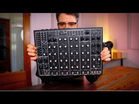
My introduction to sound design came through a Soma Pulsar 23, [Vlad Kreimer](https://somasynths.com/about-soma/)'s chaotic semi-modular synth. No manual, no background in music or DSP — just knobs labeled "envelope," "LFO," "resonance." Turn a knob, hear the change. Patch the LFO to the filter cutoff, *feel* the modulation. It's fully analog — no DAW required. Immediately intuitive, completely opaque. What was actually happening under the hood?
[](https://www.youtube.com/watch?v=PzhD7ItY0ZI)
Production was a separate quest: Ableton and Serum. Diving deeper into sound design, reading about [Pure Data](https://puredata.info/downloads/pure-data) to understand audio engineering and programming sounds. Even playing with analog synths and sequencers is basically programming loops with different basic blocks. Hardware curiosity expanded through Eurorack systems, Moog modules, the Roland 303, Teenage Engineering's EFM32 chips. Learning synths pulls you close to the building blocks: BPF, LPF, envelopes, clock, drive, LFO, VCA, wave shapes. These aren't abstract — they're the actual components.
Eventually the realization hit: **it's all the same stuff underneath**. An envelope is a multiplier that changes over time. An LFO is a slow oscillator modulating a fast one. A filter selectively removes frequencies. The Moog ladder filter and the Serum digital filter are doing the same math — one with capacitors, one with code.
Once you see sound as frequency bands that need to be filled properly, everything clicks. Sub for impact, low-mid for punch, mids for body, highs for presence. A kick drum is frequency bands layered together — a sine sub, a low-mid punch, a pitched body, a transient click. Acid squelch is a resonant filter whose cutoff moves with every note. These aren't magic tricks — they're legible, implementable, understandable.
**DSP is the fascination.** It's the layer that connects the Pulsar on my desk to the Serum plugin in my DAW to the code I'm writing. Same concepts, different implementations. This post builds a complete techno engine from that layer — where every line is visible and nothing is hidden.
```mermaid
flowchart LR
osc["Oscillators
sine, saw, square"] --> env["Envelopes
ADSR, amplitude"]
env --> filt["Filters
ladder, EQ, carve-out"]
filt --> mod["Modulation
LFOs, automation"]
mod --> gen["Generative
Euclidean patterns"]
gen --> mix["Mixing
sidechain, multiband"]
mix --> arr["Arrangement
sections, transitions"]
arr --> master["Master
compression, limiting"]
classDef default fill:#f8f8f8,stroke:#333,stroke-width:1px,color:#222
```
The engine now has 8 genre presets (acid, dark, melodic, industrial, rave, nocturne, hardgroove, hypnotic) and a companion analyzer that reverse-engineers real MP3s into the same parameter-vector structure. But it started with the question: what's actually happening when I turn this knob?
## What this covers
- **Part 1**: DSP fundamentals — samples, oscillators, aliasing
- **Part 2**: The voice — envelopes, filters, the acid squelch
- **Part 3**: Modulation — envelopes vs LFOs, signal flow
- **Part 4**: Generative structure — Euclidean rhythms, patterns
- **Part 5**: Mixing — sidechain, multi-layer kick, rumble
- **Part 6**: Arrangement — sections, transitions, full tracks
- **Part 7**: Verification — spectral analysis, dynamics, stereo
- **Part 8**: 3-band bass — sub, mid, top with per-band sidechain
- **Part 9**: Arrangement polish — automation, transitions, bleed
- **Part 10**: Reverse engineering sound — analyzer, corpus mining
- **Part 11**: Kick design — seeing the waveform, frequency layers
## Part 1: DSP fundamentals
### Audio as numbers
Digital audio is a stream of numbers, played 44,100 times per second. Each number (a *sample*) represents the air-pressure offset at that instant, between `-1.0` and `+1.0`. A WAV file is just this stream with a small header.
A one-second sine wave at 440 Hz (the A above middle C) is:
```python
import numpy as np
t = np.arange(44100) / 44100 # time in seconds
sine = np.sin(2 * np.pi * 440 * t)
```
That's it. Everything else in the stack — synths, filters, reverbs, entire tracks — is transformations of arrays like this.
### Oscillators beyond the sine
Real synths use sawtooth and square waves because they're spectrally rich (lots of harmonics the filter can carve into). The naive implementation looks like:
```python
# Naive sawtooth
phase = np.cumsum(2 * np.pi * freq / SR)
naive_saw = 2 * ((phase / (2 * np.pi)) % 1.0) - 1.0
```
This works but it **aliases** — the discontinuity at each wrap produces infinite harmonics, which reflect back into the audible range above Nyquist (half the sample rate) and cause a characteristic high-frequency hash.
The aliasing is visible in the spectrum — naive saws dump energy all the way past Nyquist, where it reflects back down into the audible range as harmonic hash:

The fix is PolyBLEP: subtract a small polynomial "bump" around each discontinuity so the step becomes spectrally well-behaved:
```python
def polyblep_saw(t, dt):
saw = 2.0 * t - 1.0
# Near t=0 (just after wrap)
m1 = t < dt
if np.any(m1):
tt = t[m1] / dt[m1]
saw[m1] -= tt + tt - tt*tt - 1.0
# Near t=1 (just before wrap)
m2 = t > (1.0 - dt)
if np.any(m2):
tt = (t[m2] - 1.0) / dt[m2]
saw[m2] -= tt*tt + tt + tt + 1.0
return saw
```
One function, ~10 lines, and your oscillators stop hashing. This is the kind of thing that separates a "numpy toy" from a real synth.
### Supersaw
Stack seven of these PolyBLEP saws, detune them in cents (each at a slightly different frequency), and randomize their start phases. The result is the signature "supersaw" sound — fat, wide, the foundation of trance/melodic-techno leads and pads:
```python
def supersaw(freq_arr, rng, num_voices=7, detune_cents=18.0):
out = np.zeros_like(freq_arr)
for i in range(num_voices):
cents = -detune_cents + 2*detune_cents*i / (num_voices-1)
f = freq_arr * (2 ** (cents / 1200.0))
phase = rng.uniform(0, 2*np.pi) + np.cumsum(2*np.pi*f/SR)
t = (phase / (2*np.pi)) % 1.0
out += polyblep_saw(t, f/SR)
return out / np.sqrt(num_voices)
```
Each voice is cheap. Seven voices with random start phases are what create the stereo width (phase differences translate to spectral width the ear hears as spaciousness).
## Part 2: The voice — envelopes and filters
### ADSR envelopes
Every note you play has *shape* over time. You pluck a guitar string: it attacks fast, decays quickly, sustains at some level while held, then releases when let go. That's ADSR — attack, decay, sustain, release — a piecewise function applied to the amplitude of a sound:

For a 303 acid line, the amp envelope is short and punchy: ~2ms attack, ~60ms decay, low sustain (0.35), ~40ms release. That's what gives each note its "pluck."
But the *acid* sound is a different envelope entirely: the **filter** envelope. The TB-303's signature is that on every gated note, its lowpass filter's cutoff frequency exponentially decays from some peak down to its baseline. That sweep is what makes the "wow" you hear.
```python
# Filter envelope per gate: exponential decay from peak to 0
for step in gated_steps:
decay_sec = 0.18 if not accent else 0.12
decay_n = int(decay_sec * SR)
env = np.exp(-np.linspace(0, 5, decay_n))
peak = 1.0 if not accent else 1.6
filt_env[step_pos:step_pos + decay_n] = env * peak
```
Accents push the peak higher AND make it faster — that's why accented notes sound brighter AND bite.
### Filters
The Moog ladder filter is a four-pole resonant lowpass. In its simplest form:
```python
for i in range(n):
g = 1 - np.exp(-2*np.pi*f[i]/SR) # cutoff coefficient
# feedback with tanh saturation (the 303 squelch lives here)
inp = tanh(x[i] - r[i] * s4)
s1 += g * (inp - s1)
s2 += g * (s1 - s2)
s3 += g * (s2 - s3)
s4 += g * (s3 - s4)
out[i] = s4
```
Four cascaded one-pole LP filters, with a tanh nonlinearity in the feedback path. The feedback is what creates resonance — as `r` approaches 4, the filter self-oscillates (becomes a sine at the cutoff frequency). The tanh is what gives the 303 its characteristic rubbery, asymmetric distortion.
Resonance is visible in the frequency response as a growing peak right at the cutoff frequency:

A cleaner version (Huovilainen 2004) puts the tanh on **every stage's input**, not just the feedback. Costs one extra tanh() per sample, gives you a more realistic 303 timbre.
Here's what a two-beat acid bassline looks like in the time domain — each note's filter envelope creates the characteristic "wow" sweep, and the amplitude tail decays through each step:

## Part 3: Modulation — envelopes vs LFOs
This is the single concept beginners get most tangled on, so it's worth being explicit.
**Envelopes and LFOs are both modulators** — neither is "the input." The signal chain has three roles:
```mermaid
flowchart LR
OSC[Oscillator
Source] --> FILT[Filter
Processor] --> AMP[Amp
Processor] --> OUT[Output]
ENV1[Env] -.->|cutoff| FILT
ENV2[Env] -.->|level| AMP
LFO[LFO] -.->|cutoff| FILT
```
- **Sources** produce audio: oscillators, noise.
- **Processors** shape audio: filters, amps, distortion.
- **Modulators** produce control signals, not audio: envelopes, LFOs. They don't live in the audio path — they get **routed** to the knobs on sources and processors.
The difference between an envelope and an LFO:
| | Envelope | LFO |
|---|---|---|
| Fires when? | Once per note (gate on) | Continuously, always running |
| Shape | One-shot: rise → fall → end | Periodic: sine / triangle / saw |
| Typical rate | ms to ~1 second | 0.1 Hz to ~20 Hz |
| Used for | Per-note shape (pluck, filter bite) | Slow breathing, vibrato, tremolo |
Visually, over the same 4-second window:

The envelope fires a new "pluck" every half-second (each note), while the LFO just cycles regardless of whether notes are playing.
In our acid voice:
- **Envelope on filter cutoff** = the per-note squelch bite
- **Envelope on amp** = the ADSR shape of each note
- **LFO on filter cutoff** = slow breathing across bars (the filter "opens up" over 7 seconds)
All three target the same parameter (cutoff) and sum. That's the modulation matrix mental model: **modulators produce control signals; patching decides what they modulate.**
## Part 4: Generative structure
### Euclidean rhythms
Random gate patterns sound random. Real grooves are *distributed*. Euclidean rhythms distribute `k` pulses over `n` steps as evenly as possible, producing rhythms that are musically satisfying for free:
```python
def euclidean_rhythm(k: int, n: int, rotate: int = 0) -> list[bool]:
pattern = [False] * n
for j in range(k):
pattern[(j * n) // k] = True
r = rotate % n
return pattern[-r:] + pattern[:-r] if r else pattern
```
The output of `E(k, n)` covers a surprising amount of world music for free:
| Pattern | Result |
|---|---|
| `E(3, 8)` | Tresillo (Cuban son clave) |
| `E(5, 8)` | Cinquillo |
| `E(7, 16)` | Acid shuffle |
| `E(9, 16)`, `E(11, 16)`, `E(13, 16)` | Dense techno grooves |
For acid we pick randomly from `{9, 11, 13}` pulses over 16 steps. The groove is built-in; we don't have to "compose" it.
Here's what those three look like — each row is a 16-step bar, filled circles are pulses:

### LFO automation across the render
The single biggest upgrade from "loop" to "interesting loop" is a slow LFO on the filter cutoff:
```python
# One full LFO cycle across the entire render
lfo_rate = 1.0 / total_render_seconds
lfo = np.sin(2 * np.pi * lfo_rate * t_sec)
base_cutoff_swept = base_cutoff * (1.0 + 2.0 * depth * lfo)
```
A 4-bar loop with LFO modulation feels alive in a way that the same 4 bars *without* modulation feel robotic. The spectral centroid of our test output swept from 820 Hz to 11 kHz across a 7-second render — that's the LFO "opening up" and closing the filter over time.
## Part 5: Mixing and production
### Sidechain ducking — THE techno trick
Every time the kick hits, duck the bassline's amplitude down ~6 dB for ~200 ms, then exponentially recover. This is the single biggest "this sounds like real techno" upgrade.
Visually, the bass gain envelope dips sharply at each kick and exp-recovers before the next:

The two curves show the same floor (0.4, ~-8dB) but different attack times — the dotted green line is the slower "musical" attack used in the melodic preset. You can see how the bass initial transient comes through before ducking begins.
Implementation:
```python
def sidechain_envelope(n, kick_positions, floor=0.4,
attack_s=0.005, release_s=0.22):
env = np.ones(n)
attack_n = int(attack_s * SR)
release_n = int(release_s * SR)
shape = np.ones(attack_n + release_n)
shape[:attack_n] = np.linspace(1.0, floor, attack_n)
rel_t = np.linspace(0, 5, release_n)
shape[attack_n:] = 1.0 - (1.0 - floor) * np.exp(-rel_t)
for pos in kick_positions:
end = min(pos + len(shape), n)
env[pos:end] = np.minimum(env[pos:end], shape[:end - pos])
return env
```
The **attack time** matters a lot for character:
| Attack | Feel |
|---|---|
| 1–5 ms (surgical) | Clean separation, "robotic" pump — dark techno |
| 10–30 ms (musical) | Classic 909 pump-and-breathe feel — house, melodic |
| 50–100 ms | Loses the pump; more like general compression |
Melodic techno specifically benefits from 20–30 ms attack because the first "thump" of the bass comes through before ducking starts — that's what makes the track *breathe*.
### The modern hard-techno kick
A kick from a modern hard-techno production isn't a single sample — it's a **stack**:
```mermaid
flowchart TB
subgraph KICK[Multi-layer kick]
SUB[Sub layer
sine ~45 Hz
~200ms tail]
BODY[Body layer
pitched sine + FM modulator
distorted]
CLICK[Click layer
noise burst + 3.2kHz ping
beater transient]
end
BODY --> SAT1[Soft clip
tanh]
SAT1 --> SAT2[Asymmetric
tube-ish]
SAT2 --> SAT3[Hard clip
~-1 dBFS]
SUB --> MIX[Sum: 42% sub + 45% body + 18% click]
SAT3 --> MIX
CLICK --> MIX
MIX --> LIM[tanh limiter]
LIM --> OUT[Kick output]
```
- **Sub** gives weight (20–80 Hz, clean sine, tight decay).
- **Body** gives the thump (80–120 Hz, pitch-swept, heavily distorted).
- **Click** gives the beater transient (2.5–4 kHz, very short).
- **Three saturation stages** create harmonic density without muddying the sub.
That's why a properly-layered kick translates on tiny laptop speakers AND on club soundsystems — different layers own different frequency bands.
The resulting waveform shows all three layers at work — sharp click transient at the start, FM-distorted body for the first ~150 ms, and the sub-sine tail continuing underneath:

### Rumble layer — the modern thunder
On top of the kick, modern hard techno often adds a **rumble layer**: another kick-timed hit, heavily distorted, aggressively lowpassed (80 Hz), and sent through a huge reverb:
```python
def render_rumble_layer(total_n, kick_positions, freq=45, amp=0.55):
dry = np.zeros(total_n)
hit = rumble_hit(freq=freq)
for pos in kick_positions:
dry[pos:pos+len(hit)] += hit
wet = simple_reverb(dry, room=0.92, damp=0.5) # huge room
wet = onepole_lowpass(wet, 85.0) # 80Hz ceiling
wet = np.tanh(wet * 2.2) # more distortion
return wet * amp
```
Because the reverb tails overlap, the result is continuous rolling low-frequency thunder — perceived as rumble, not as distinct strikes. This is the signature of modern industrial/hard techno.
## Part 6: Arrangement
A loop isn't a track. A track is a loop with *structure over time* — sections that build tension, drop, breathe, and release.
### The canonical techno structure
A techno track isn't one loop — it's a sequence of *sections*, each a multiple of 8 or 16 bars, with different voices active and different parameter values:
Each section has different voices active and different parameter values. The structure is represented as a list of `Section` objects:
```python
@dataclass
class Section:
kind: str # 'intro' / 'build' / 'main' / 'break' / 'outro'
bars: int
mute_bass: bool = False
mute_kick: bool = False
mute_hats: bool = False
filter_mult: float = 1.0 # scales base filter cutoff
reverb_mult: float = 1.0 # scales reverb send
voice_gain: float = 1.0
transitions: tuple = () # ('riser', 'impact', 'roll')
transition_bars: float = 2.0
```
### Three genre arrangements
Same framework, different shapes:

Notice how **melodic** has the longest breakdown (~63s) — that's the emotional core of the genre. **Dark** has the longest intro (~58s) — the genre rewards patience, slowly building from just a noise bed. **Acid** is the most symmetric — it's the most "functional" of the three, designed for dance-floor progression.
### Transitions — the glue
Between sections, three production elements tie everything together:
```mermaid
flowchart LR
BUILD[Build section
last N bars] --> RISER[Riser:
filtered noise
sweeping up]
BUILD --> ROLL[Snare roll:
accelerating 16ths
to 64ths]
BREAK[Break end
last 1 bar] --> IMPACT[Reverse reverb
swelling INTO
downbeat]
RISER --> MAIN[Main section
starts full-force]
ROLL --> MAIN
IMPACT --> MAIN
```
The **riser** is filtered white noise whose cutoff AND amplitude both rise exponentially over 2–4 bars. The moog_ladder's resonance gives it that whistling, tension-laden character.
The **impact** is noise rendered forwards (noise-burst with decaying lowpass), then *reversed*. What the listener hears is a swell that "sucks them into" the downbeat of the next section.
The **snare roll** is accelerating percussion — starting at 8th-notes, each hit shortens the next interval by 12%, down to 64th-notes by the end.
### Master bus
After sections are concatenated, the final pipeline:
```mermaid
flowchart LR
CONCAT[Crossfade-concatenated
section audio] --> HPF[30Hz HPF
kills rumble]
HPF --> COMP[Bus compressor
3:1, 5ms/120ms]
COMP --> SAT[Final soft-clip
tanh * 0.9]
SAT --> NORM[Peak normalize
to -1 dBFS]
NORM --> WAV[Stereo WAV]
```
The bus compressor isn't there to make things louder — it's there to *glue*. It evens out the section-to-section level differences and gives the whole track a cohesive feel.
## Part 7: Verification — how we know it actually works
When you're iterating on synthesis code with twenty-plus per-sample loops, you can't listen to every render. A full five-minute track takes 30–120 seconds to render, and a single session produces dozens of renders as you tweak parameters. You need *programmatic* sanity checks that run in milliseconds and catch most regressions — and critically, every feature you claim to have added needs to be **measurable**, not just audibly present. If you can't measure it, you can't tell whether your next change broke it.
Here are the checks that ran at every step of this project, and the discipline that made iterating fast.
### The three-line integrity check
Runs after every render. Catches 90% of the ways audio code goes wrong:
```python
import wave, numpy as np
w = wave.open(path)
s = np.frombuffer(w.readframes(w.getnframes()), dtype=np.int16)
s = s.reshape(-1, 2).astype(np.float32) / 32768.0
assert not np.any(np.isnan(s)), "NaN in output"
assert np.max(np.abs(s)) < 1.0, "clipping"
assert np.sqrt(np.mean(s**2)) > 0.05, "silent output"
```
NaN usually means a division-by-zero or `log(0)` in a filter. Clipping means a missed normalization step. Silent output means a voice isn't reaching the mix. All three are catastrophic, all three are instantly detectable.
### Spectral distribution — does each preset match its genre signature?
Every preset has an expected spectral signature. Dark should have roughly 3× the sub energy of acid. Melodic's rolling bass should live in the 80–300 Hz pocket:
```python
mono = s.mean(axis=1)
spec = np.abs(np.fft.rfft(mono))
freqs = np.fft.rfftfreq(len(mono), 1/44100)
for name, lo, hi in [("sub", 20, 80), ("low", 80, 300),
("mid", 300, 2000), ("hi", 2000, 22000)]:
ratio = spec[(freqs >= lo) & (freqs < hi)].sum() / spec.sum()
print(f" {name}: {ratio:.3f}")
```
When rolling bass was added to the melodic preset, its 80–300 Hz band jumped from 0.111 to 0.138 — matching intent. If that number had stayed flat, something in the mixing pipeline would have been swallowing the new voice before it hit the WAV.
### Stereo width
Stereo output requires a different check:
```python
l, r = s[:, 0], s[:, 1]
corr = np.corrcoef(l, r)[0, 1] # 1.0 = pure mono, 0.0 = decorrelated
side = (l - r) / np.sqrt(2)
mid = (l + r) / np.sqrt(2)
width = np.sqrt(np.mean(side**2)) / np.sqrt(np.mean(mid**2))
```
For the melodic preset: `corr=0.96, width=0.14`. For acid: `corr=0.99, width=0.02`. The numbers match the design intent: melodic is wide (stereo supersaw pad), acid stays narrow (303 is a mono instrument).
This same measurement caught a bug where a refactor accidentally collapsed the stereo pad back to mono — `width` dropped from 0.14 to 0.02. Caught in seconds, not hours.
### Per-section dynamics — does the track actually breathe?
A full arranged track should have audible dynamic variation. The break should be quieter than the main. The outro should ramp down:
```python
bar_n = int(60 / bpm * 4 * 44100)
for name, start_bar, end_bar in section_ranges:
seg = mono[start_bar * bar_n : end_bar * bar_n]
rms = np.sqrt(np.mean(seg**2))
print(f" {name}: rms={rms:.3f}")
```
Expected output for melodic:
```
main1: rms=0.401
break: rms=0.197 ← kick drops out; ~50% of main's energy
main2: rms=0.400
```
If the break section's RMS is the same as main's, the kick-mute logic isn't working. If main2 is dramatically quieter than main1, the peak normalization is miscalibrated for a low-energy section pulling the whole track down.
### Verifying specific features fire
The most important habit: when you add a feature, instrument it directly, not just through its audible output.
**Pattern variations** — does `apply_pattern_variations` actually produce different bars?
```python
base = generate_pattern(rng, ACID_PRESET)
varied = apply_pattern_variations(base, 16, rng)
for b in range(16):
bar = varied[b*16 : b*16 + 16]
gates = [i for i, s in enumerate(bar) if s.gate]
accents = [i for i, s in enumerate(bar) if s.accent]
print(f"bar {b:2}: gates={gates} accents={accents}")
```
Output shows bar 4 dropping one gate, bar 10 gaining an accent, bar 12 dropping a gate entirely. Variations confirmed firing — deterministically, so the same seed produces the same variations every time.
**Sidechain envelope** — does the ducking curve match what we designed?
```python
positions = [int(SR * t) for t in [0.0, 0.5, 1.0, 1.5]]
env = sidechain_envelope(total_n, positions, floor=0.4,
release_s=0.22, attack_s=0.005)
for dt in [0.001, 0.01, 0.05, 0.1, 0.15, 0.2, 0.25]:
print(f"t=+{dt:.3f}s env={env[int(dt*SR)]:.3f}")
```
Expected (and measured) shape:
```
t=+0.001s env=0.879 ← just started attacking
t=+0.010s env=0.465 ← at/near floor
t=+0.050s env=0.784 ← exp-recovering
t=+0.100s env=0.931
t=+0.250s env=1.000 ← fully recovered
```
The measurement confirms the envelope reaches the floor (0.4) around 10 ms, then exponentially recovers to 1.0 over 250 ms. If any of those numbers drifted, the sidechain would be either too tight (kick-bass fight) or too loose (audible pumping).
### The discipline
Every change had a measurement behind it:
1. **Design a measurable claim.** "Dark should have ~3× the sub energy of acid." "Stereo width should be measurable in the output." "The sidechain envelope should dip to 0.4 within 10 ms of each kick."
2. **Ship the feature.**
3. **Measure.** Does the number match the claim?
4. **Only then listen** — to confirm the subjective experience matches the measurable one.
This is what makes shipping twenty commits in a few days tractable. When something breaks, you know within thirty seconds because a known-good number moved in the wrong direction. The listening step is for catching things measurement can't — a filter setting that's *technically correct* but sounds sterile, an arrangement that's *dynamically varied* but emotionally flat. Measurement catches the regressions; ears catch the taste.
One more habit worth mentioning: **keep a small test script** that renders a representative 2-bar loop of each preset and prints the standard checks. It runs in 10–15 seconds end-to-end and can be re-run after any change. Not a formal test suite — just a quick `is-my-numpy-code-still-doing-the-thing` script. In practice this replaces 80% of "load the WAV into a DAW and hunt for the bug" sessions.
## Part 8: Frequency bands and the 3-band bass architecture
Mixing the low end of an electronic track is less about choosing nice-sounding bass synths and more about *frequency discipline* — making sure every element has its own pocket in the spectrum and nothing's fighting for the same Hz.
This band-based thinking shows up everywhere. The Pulsar 23 separates voices into BD (bass drum), Bass, SD (snare), HHT (hi-hat) — each in its own frequency range. The Allen & Heath Xone:96 mixer gives you Low, Mid, Mid/High, High EQ bands. Same concept: divide sound into frequency buckets, shape each one independently.
The standard audio frequency map, divided the way mixing engineers actually think about it:
| Band | Range (Hz) | What lives there | Common mixing decisions |
|---|---|---|---|
| **Deep sub** | 20 – 40 | Room-shaker fundamentals | Often HPF'd to 30 Hz — inaudible on most systems, eats headroom |
| **Sub** | 40 – 90 | Kick fundamental, sub-bass sine | Keep mono; this is where club systems translate |
| **Low** | 90 – 200 | Kick body, bass-note fundamentals | Where "weight" lives |
| **Low-mid** | 200 – 500 | Mid-bass body, "mud zone" | Surgical cuts here keep the mix clean |
| **Mid** | 500 – 2000 | Bass growl, vocal formants, synth body | The "presence" pocket — melodic-techno sweet spot at 800 Hz |
| **Mid-high** | 2000 – 5000 | Hi-hat/clap bodies, kick click, attack transients | Where "snap" lives |
| **High** | 5000 – 12000 | Hat/cymbal air, pad shimmer | Too much = fatiguing |
| **Air** | 12000 – 20000 | Open-hat sibilance, reverb sheen | Rolls off gently for warmth |
Once you see the track through this lens, the single biggest technique for a clean low end becomes obvious: **split the bass into three bands, each with its own synthesis, its own filter, and its own sidechain depth.** This is what separates "a bass synth that sounds OK solo" from "a low end that translates on every system."
### The three layers
```mermaid
flowchart TB
subgraph SUB[Sub-bass layer — 40-90 Hz]
S1[Pure sine at chord root
-2 octaves below voicing]
S2[Phase-locked to kick
triggered on each kick hit]
S3[LP-only content
no harmonics, mono-center]
end
subgraph MID[Mid bass layer — 100-500 Hz]
M1[PolyBLEP saw at chord root
-1 octave below voicing]
M2[Resonant LP at ~550 Hz
+3 dB peak at 160 Hz]
M3[Dense 16th-note rolling pattern
HPF 100 Hz to clear sub]
end
subgraph TOP[Top bass layer — 300-1500 Hz]
T1[Saw + triangle at chord voicing]
T2[HPF 300 Hz + LPF 1500 Hz
+4 dB peak at 800 Hz]
T3[Staccato envelope
Haas-widened stereo]
end
SUB --> DUCK_SUB[duck floor 0.22
hardest pump]
MID --> DUCK_MID[duck floor 0.38
standard pump]
TOP --> DUCK_TOP[duck floor 0.65
rides above the duck]
DUCK_SUB --> MIX[Summed stereo mix]
DUCK_MID --> MIX
DUCK_TOP --> MIX
```
Each layer plays the *same note* (chord root) but in a different register and with a different sidechain depth. Three things at once in the low end, not fighting, each doing what it's best at:
- **Sub** handles weight. Nothing above 90 Hz. Ducks hardest so the kick transient punches through clean.
- **Mid** handles warmth / body. HPF at 100 Hz means it physically cannot muddy the sub. The 160 Hz peak is the classic melodic-techno "body" boost.
- **Top** handles presence / groove. HPF at 300 Hz strips everything below — this layer's job is to move, not to thump. Ducks lightest so it keeps driving even when kick-bass is ducked heavily.
The sidechain-depth differentiation is the detail most tutorials miss. A single sidechain envelope applied uniformly flattens the bass into one ducked blob. Three different depths preserve the **illusion of three separate instruments** even though they're all following the same chord progression.
### Breakdown: swap the mid for a reese
During the breakdown, where the kick drops out and tension needs somewhere to live, melodic techno swaps the rolling mid-bass for a **reese bass**:
```python
# Two sawtooth oscillators with LFO-modulated detune (±15 cents @ 0.3 Hz)
f1 = freq * (2 ** (+detune_semi / 12)) # → left channel
f2 = freq * (2 ** (-detune_semi / 12)) # → right channel
# Each channel filtered through moog ladder separately
# Sustained per-bar envelope (150 ms attack, holds, 250 ms release)
```
The defining feature is the time-varying detune — two saws slowly drifting in and out of phase with each other. Their beating pattern is what creates reese's growling, metallic quality. Sending each saw to a different channel makes the beating happen *across the stereo field* rather than summed mono, which is how real reese gets its width.
### Vocal chops — the ghost vocal without vocals
One more element that lives mostly in the 500-3000 Hz band: the atmospheric "ghost vocal" chop that appears on almost every melodic-techno track. You can synthesize it without any vocal samples:
```python
# Carrier: saw at chord voicing + 12 semitones (vocal range ~260-520 Hz)
# Three biquad_peak bell filters at vowel formant positions
voiced = biquad_peak(saw, 650, gain_db=14, q=5.5) # formant 1
voiced = biquad_peak(voiced, 965, gain_db=12, q=5.0) # formant 2
voiced = biquad_peak(voiced, 2425, gain_db=10, q=4.0) # formant 3
# HPF 250 Hz strips fundamentals — only formant content
# 8th-note rhythmic gate at depth 0.95 (hard on-off chops)
# Haas-widen for stereo spread, send to reverb
```
Three resonant peaks at vowel-formant positions tell the ear "this is a voice" even though no voice has ever been recorded. Averaging the formants of "ah" (730 / 1090 / 2440) and "oh" (570 / 840 / 2410) gives a neutral vowel that morphs well through chord changes.
### Melodic-techno bass sweet spots — two biquad peaks you always want
Two surgical peak EQs consistently show up in melodic-techno bass production:
- **+3 dB @ 160 Hz (Q 0.8)** on the mid-bass layer — adds body/warmth
- **+4 dB @ 800 Hz (Q 0.9)** on the top-bass layer — adds growl/presence
These aren't arbitrary. 160 Hz is the bottom octave of bass-note fundamentals (MIDI 43-55 range = 98-195 Hz); boosting there fattens every note. 800 Hz is where the bass's upper harmonics stack — boosting makes the bass "talk" (cut through a busy mix, read as present on small speakers).
Both are implemented as RBJ-cookbook peaking biquads — ~15 lines of NumPy each:
```python
def biquad_peak(x, freq_hz, gain_db, q=1.0):
A = 10 ** (gain_db / 40)
w = 2 * np.pi * freq_hz / SR
alpha = np.sin(w) / (2 * q)
b0 = 1 + alpha * A
b1 = -2 * np.cos(w)
b2 = 1 - alpha * A
a0 = 1 + alpha / A
a1 = -2 * np.cos(w)
a2 = 1 - alpha / A
# ...biquad direct-form-I loop
```
## Part 9: Arrangement polish — automation, transitions, bleed
The basic arrangement framework from Part 6 has each section render as a self-contained block with constant parameters. For a full-sounding track, each section needs three more things:
### Intra-section automation curves
A "build" section with constant parameters is indistinguishable from "the main, but quieter." To feel like an actual *build*, parameters need to ramp *within* the section:
```python
Section("build", bars=16,
voice_gain=0.55, voice_gain_end=1.0, # ramp 55% -> 100%
reverb_mult=1.0, reverb_mult_end=1.8, # reverb swells
transitions=("whoosh", "gap"), transition_bars=4)
```
Linear ramps in `voice_gain_end` and `reverb_mult_end` produce per-sample curves applied to every melodic voice (bass, rolling, reese, top_bass, vocal_chop, sub_bass). The build now *builds*: bass opens up, reverb swells, culminating in the whoosh + gap that delivers the drop.
### Transition elements — riser / impact / roll / whoosh / gap
Four transition types fire in the last `transition_bars` of a section:
| Transition | Shape | Use |
|---|---|---|
| `riser` | Filtered white noise with exponentially rising pitch + amplitude | Generic build transitions — all presets |
| `impact` | Noise burst rendered forwards, then reversed | Short (1 bar) pre-drop hit |
| `whoosh` | Descending-cutoff filtered noise through reverb, reversed | Long (4-bar) melodic-techno pre-drop swell |
| `gap` | Muted dry content for the final half-bar | Pre-drop silence (reverb tails still ring) |
One transition type didn't survive listening tests: an accelerating "snare roll" that progressed from 8th notes to 32nd notes across the build. The accelerating hits consistently read as a stutter or glitch rather than a musical intensification, regardless of preset. Cutting features that *look* right on paper but don't hold up audibly is part of the discipline.
### Reverb-tail bleed between sections
The biggest arrangement bug for this project, silently swallowed by the 80 ms crossfade: when a heavily-reverbed breakdown ends, its reverb tail is **cut**, not allowed to bleed into the next section. Listeners perceive this as an abrupt stop.
Fix: render each section with `bars + tail_bars` worth of samples. During the tail, voices/drums are zero (already faded out), but the delay and reverb lines continue processing and produce a naturally decaying tail. Then concatenate sections with **additive overlap** (sum, not crossfade) over `tail_bars`:
```python
def tail_overlap_concat(parts, tail_n):
active_lens = [len(p) - tail_n for p in parts]
total = sum(active_lens) + tail_n
result = np.zeros((total, 2), dtype=np.float32)
pos = 0
for i, part in enumerate(parts):
result[pos:pos + len(part)] += part
pos += active_lens[i]
return result
```
Section N's reverb tail now rings through the first bar of section N+1. Breaks no longer end with a hard cut.
### Multiband master automation
The tutorial-3 trick: at the breakdown, **remove the sub frequencies** (not via drop in gain, via actual HPF). This creates "space" — the kick drops out, and the entire low-frequency spectrum goes with it. When the kick returns at the drop, the re-introduction of sub content is dramatic even if the drum pattern is the same:
```python
Section("break", bars=32, mute_kick=True, reverb_mult=2.2,
use_reese_bass=True,
low_cut_hz=180.0) # HPF at 180 Hz for the whole section
```
Implemented as a one-pole HPF / LPF applied to the final stereo mix in the last step before normalize. Zero means "off" (no filtering). Enabled on melodic's break section for tension.
## Part 10: Reverse engineering sound
Building a generator is one thing. **Knowing whether it sounds like real techno** is a different problem — you can hand-tune sidechain release forever without ever asking whether real tracks use 200 ms or 350 ms.
Audio analysis can extract the DNA of a track: tempo, key, arrangement structure, frequency content, rhythmic patterns. The same techniques power everything from DJ software (beat detection, key matching) to remix tools (stem separation) to streaming recommendations (genre classification).
### What audio can actually tell you
Given an MP3, you can extract:
| Measurement | What it reveals |
|---|---|
| Tempo + beats | BPM, downbeat position, bar boundaries |
| Key | Root note + scale (major/minor) |
| Chord roots | Per-bar harmonic progression |
| Sub-bass pitch | Pedal bass patterns vs. changing roots |
| Onset density | Activity level per frequency band |
| Section boundaries | Where intros, builds, drops, breaks occur |
| Stereo width | Correlation + side/mid ratio per section |
| Swing ratio | How much the groove deviates from straight 16ths |
| Measurement | Technique |
|---|---|
| Tempo + beats | `librosa.beat.beat_track` (autocorrelation on onset envelope) |
| Key | Cosine similarity of averaged chromagram against Krumhansl-Schmuckler major/minor profiles (all 24 keys scored symmetrically) |
| Per-bar chord root | Chromagram window argmax per bar |
| Per-bar chord quality | Template matching against maj/min/sus/dim/maj7/min7 rotated through 12 roots |
| Section boundaries | `librosa.segment.agglomerative` on mel-spectrogram features, clustered into ~7 segments |
| Sub-bass pitch track | FFT-isolated 30-120 Hz band, then chromagram on the low-passed signal — independent of chord chromagram, reveals pedal-bass patterns |
| Stereo width | L-R correlation + side/mid RMS ratio per section |
| Swing ratio | Median offset of odd-vs-even 16th-note hat onsets from the strict grid |
| Onset density | Band-limited onset detection in 5 frequency ranges |
### The 10-track reference corpus
Running this on a set of modern-techno reference tracks across multiple sub-genres (melodic-progressive, hypnotic, hard techno, minimal, acid, mid-tempo electronica) produced the following comparative data, which drove many of the preset-tuning decisions:
| # | Genre | BPM | Key | Break | Sub onsets/min | Swing |
|---|---|---|---|---|---|---|
| 1 | melodic-progressive (short-format) | 129 | Cm | 1 bar | 788 | 0.55 |
| 2 | melodic-progressive (modular) | 126 | Cm | 7+7 bars | 670 | 0.50 |
| 3 | hypnotic | 129 | Cm | 7 bars | 496 | 0.50 |
| 4 | hypnotic (alt.) | 129 | Fm | 2 bars | 673 | 0.55 |
| 5 | minimal / high-tech | 126 | Fm | — | 620 | 0.50 |
| 6 | hard techno (collab) | 140 | Am | **0 bars** | 1014 | 0.61? |
| 7 | hard techno | 140 | F#m | 15+15 (staged) | 792 | 0.50 |
| 8 | hard-groove / tech-house | 131 | F#m | — | 1127 | 0.50 |
| 9 | acid | 136 | D#m | 1 bar | 811 | 0.53 |
| 10 | mid-tempo electronica | 123 | F#m | — | 933 | 0.50 |
### What 10 tracks taught us
**Every track is in a minor key** — 100%.
**BPM clusters are real** — two gravity wells at 126-129 (melodic/hypnotic) and 139-140 (hard techno).
**F# minor is the most common key** (4/10 tracks).
**Swing is bimodal** — tracks are either dead straight (0.500) or softly swung (0.53-0.55).
**Break length inversely correlates with BPM.** Melodic tracks have long breaks; hard techno has 0-2 bar breaks.
**Bass drones are universal.** Most tracks hold the root note for 14-27 bars before any chord change.
### Where audio analysis hits its ceiling — the MIDI reveal
Audio analysis has limits. MIDI tells the truth:
| Measurement | MIDI ground truth | Audio can see |
|---|---|---|
| Tempo | **128.00 BPM** | 129.20 BPM (-1.2 off) |
| Layers | **17 named tracks** | blended signal |
| SAW lead | **4 notes in 7+ min** | not detectable |
| Chord voicing | **Cm7 (C-Eb-G-Bb)** | root detected, 7th ambiguous |
| Doubling | SYNTHBASS×2, TRUMPET×3 | hears "thick" or "wide" |
**Biggest lesson: hypnotic-techno leads are minimal.** The SAW track played only 4 notes in 7 minutes. Generators often overproduce — restraint is harder to algorithmize than density.
### The doubling trick
Real productions double instruments — multiple tracks with identical patterns at different octaves or with different processing. Audio analysis can't see separate layers; you just hear "a thick synthbass" or "a wide trumpet." Width through stacking, not single-pass rendering.
## Part 11: Kick design — seeing the waveform
Kick design is a fun exercise because kicks make such a massive difference in how a track feels. And they need to lock with the bassline — the fundamental frequencies, the decay times, the punch. Get the kick right and the whole track sits. Get it wrong and nothing else matters.
A kick drum is frequency bands layered together. Here's what that looks like:

The visual tells the story: a sharp transient (click), a pitched sweep (body), and a sustaining fundamental (sub). Building this in NumPy means understanding which frequency bands create which perceptual qualities.
### The multi-layer architecture
Starting from scratch, a naive kick is a single sine with a pitch envelope:
```python
freq = low + (high - low) * np.exp(-t * pitch_decay)
body = np.sin(2*pi*np.cumsum(freq)/SR)
env = np.exp(-t * amp_decay)
return body * env
```
This sounds like a kick but feels thin. The missing ingredients are frequency bands:
| Layer | Frequency range | Perceptual contribution |
|-------|----------------|------------------------|
| Sub | 40-55 Hz | Chest impact, room-shake |
| Low-mid | 80-150 Hz | Punch, weight |
| Body | 200-500 Hz | Pitch sweep, character |
| Click | 2-5 kHz | Attack, transient definition |
Each band is a separate sine oscillator with its own envelope. Summed together, they create a kick that hits across the entire frequency spectrum.
### Adding weight
A thin kick lacks low-mid energy. Adding a layer at twice the fundamental (the first harmonic) fills the 80-200 Hz "punch pocket." The body envelope needs to decay slower — a heavy techno kick rings for 400-500 ms, not 200 ms.
Weight also comes from saturation. Running the summed layers through soft clipping, then asymmetric clipping, then hard clipping adds harmonic content that makes the kick feel larger without raising its fundamental frequency.
### Adding punch
Weight isn't punch. Punch comes from the first 15 milliseconds — the transient. Multiply this portion by 1.5× and you feel the kick **hit** rather than just play.
Post-kick compression adds density: a fast peak compressor applied to each kick hit (not the master bus) "smashes" the dynamics so the kick sits tighter in the mix. The attack is fast enough to let the transient through before clamping; the release matches the kick's natural decay.
The EQ curve matters too. A single boost at 80 Hz is vague. Two peaks at 50 Hz (room-shake) and 100 Hz (chest-punch) hit both targets cleanly.
### Aggression without aliasing
Pushing drive creates harmonics, but too much drive pushes harmonics above Nyquist where they fold back into the audible range. The folded harmonics beat against the fundamental — you hear it as "vibration" instead of "hardness."
The fix is disciplined gain staging. Two saturation stages with moderate drive produces cleaner harmonic content than one stage with extreme drive. And reverb tails need exponential release curves, not linear fades, or you get clicks at the gate closure.
### What the waveform teaches
Looking at a kick waveform shows you exactly what's happening: the initial click width tells you about the transient, the decay slope tells you about the envelope, and any ringing tells you about resonance issues. When a kick sounds "wrong," plot the waveform — the problem is usually visible before you can name it.
## Genres as frequency distributions
A genre isn't a different synthesis method — it's a different distribution of energy across frequency bands. The same DSP engine produces eight different genres just by reweighting the bands:

Dark techno has **~3.7× the sub energy** of acid. That's not a different architecture — it's a rumble layer, a multi-layer kick, and more sub-layering all stacking in the low end. Acid's character lives in the mid/high content (the filter envelope sweeping through 500 Hz to 4 kHz per note, plus bright hi-hats). Melodic sits in between — sub from the kick, mids/highs from the supersaw arp and pad.
The presets are all the same code with different parameter vectors:
| Preset | Root | Character |
|---|------|-----------|
| `acid` | Am | Squelchy 303, hypnotic repetition |
| `dark` | Cm | Heavy, aggressive, industrial |
| `melodic` | Cm | Euphoric, rolling bass, chords |
| `industrial` | Am (low) | FM bass, metal percussion |
| `rave` | Em | 90s hoover, pitch-bent detune |
| `nocturne` | F#m | Atmospheric, swung hats |
| `hardgroove` | Bbm | Dense, narrow stereo |
| `hypnotic` | Cm | Sparse, restrained |
Change ~20 numbers and the genre changes. The DSP underneath is identical.
## Key takeaways for DSP and sound design
1. **Everything is an array of numbers between -1 and 1.** Every synth, filter, reverb, or kick drum is a transformation of those arrays. Once you see this, the mystery evaporates.
2. **Envelopes and LFOs are both modulators.** They don't sit in the audio path — they get *routed* to parameters. Patching decides what modulates what.
3. **Aliasing is the #1 thing that makes naive synths sound digital.** PolyBLEP is ~10 lines and solves 90% of it.
4. **The 303 sound is an envelope on the filter cutoff, not on the amp.** Four-pole lowpass + tanh feedback + per-note exponential filter env = acid.
5. **Sidechain ducking is the single biggest "this is techno" trick.** Without it, kick and bass fight; with it, they lock.
6. **Euclidean rhythms give you groove for free.** You don't have to compose — `E(11,16)` already swings.
7. **A loop isn't a track.** The difference is arrangement — sections with automated parameters over time, and transition elements at section boundaries.
8. **Genres are parameter vectors.** Same DSP, different numbers. Dark techno isn't "a different kind of synthesis" — it's a lower root note, darker scale, more sub, heavier drive, added rumble, and bit crush.
9. **Real techno uses restraint, not density.** MIDI analysis of a hypnotic-techno reference track revealed its lead plays *4 notes in 7 minutes*. Our generator was producing ~280. Cutting density to 50% and triggering every 8 bars approximates the real aesthetic.
10. **Kicks are multi-layer.** The difference between a thin kick and a club kick is 4 layers (sub + low-mid + body + click), each with its own envelope, summed through multi-stage saturation, through a dual-peak EQ (50 + 100 Hz), through a transient shaper, through a per-kick peak compressor, through a gated reverb. All of that is what "a good techno kick" actually is.
11. **Measure everything.** "Dry," "not heavy," "vibrating," "too clicky" — every listener complaint maps to a measurable DSP mechanism (decay envelope too fast, missing low-mid punch, Nyquist fold aliasing, excess 3 kHz content). The discipline of naming what's broken is half of fixing it.
12. **Reference tracks set objective targets.** "Does this have enough swing?" Check: real techno is 0.50 or 0.53-0.55 — pick one. "Is the breakdown too long?" Check: real 140 BPM tracks have 0-2 bar breaks. Subjective questions resolve fast when you have a corpus.
## Frequency allocation — mixing as carving space
Acid techno has a unique mixing challenge: the 303 voice and the kick both occupy the same frequency range. When they hit together, they mask each other.
What sounds like "turn it down" is actually a **frequency allocation** problem. The solution is making space, not reducing level.
### HPF carve-out
High-pass filtering the acid voice removes the low mud that competes with the kick's fundamental while leaving the squelch character intact. This is surgical EQ: you're not changing the sound, you're removing the part that doesn't serve it. The acid still sounds like acid — it just doesn't fight the kick anymore.
### Sidechain as groove
Ducking isn't just mixing — it's rhythm. Aggressive ducking creates the pumping effect that *is* the acid techno groove. The kick punches through because the acid literally gets out of its way on every beat. The sidechain envelope *is* the rhythm.
### Kick tuning tradeoffs
A deep kick (40-45 Hz) is perfect on club systems but inaudible on laptop speakers. Raising the fundamental makes it portable but loses chest-rumble. The compromise: a mid-range fundamental plus a low-mid layer for punch, with parallel saturation adding harmonic content that makes the kick feel larger without raising its frequency.
You can't have it all. Every tuning decision is a tradeoff between portability, sub presence, and punch. Seeing the frequency response helps you choose which compromise to make.
## Melody: repetition with variation
Early versions generated arpeggios that wandered indefinitely. Real techno tracks have memorable hooks — short motifs that repeat, then vary, then return.
**Bassline jumps** — static basslines get boring. Random octave and fifth intervals create forward momentum without losing the root. The pattern remains recognizable because it *mostly* stays put.
**Call/response** — a question phrase followed by an answer phrase at a different pitch. This is earworm mechanics: repetition + slight variation = memorability. The system tracks motif length and repeats before varying, so the listener learns the melody before it changes.
## Pattern generation: bounded randomness
Euclidean rhythms distribute hits evenly across a bar. This is powerful but predictable — the same pattern every time gets repetitive.
The solution is **bounded randomization**: randomly choose from a range of densities instead of fixing one. You get sparse patterns that breathe, dense patterns that drive, and everything in between. The variety makes each generation unique while staying within "sounds like techno" bounds.
## Arrangement: automation over time
A track isn't a loop repeated. The difference is **parameter automation over time**:
- **Stereo width drama** — intros and breaks are super-wide for atmosphere, mains are narrow for focus. The contrast creates energy drama without adding more sounds.
- **Per-section ramps** — parameters like reverb and voice gain fade across a section's duration. A build doesn't just add layers; it slowly increases intensity so the drop feels earned.
- **Multi-band sidechain** — low frequencies duck more than high frequencies. The kick's fundamental clears space for the bass, but the high-end sparkle stays present.
Arrangement is automated parameter change, not just layer management.
---
All of this is pure NumPy. No audio libraries for synthesis, no sample packs, no plugins. Everything you hear is math between `np.arange` and `np.tanh`. Plot the waveform and you see exactly what's happening — frequency bands, envelopes, transient shapes. The DSP is never a black box.